Introduction

Rare Events in Noisy Systems

The motivation for this work lies in improving the tools available to study rare events. Such events, which occur extremely infrequently on average, many times dictate a stochastic system’s most relevant and interesting dynamics. Everyday examples of such events include financial market crashes, earthquakes, or the failure of a mechanical part. In the natural sciences, the systems of interest are normally much smaller in scale, for example the study of activated chemical reactions, polymer dynamics or the configurational change of (relatively large) proteins in biological systems.

As the name rare event suggests, the dynamics driving these systems is dominated by the large chunks of time in which no abnormal events occur. The disparity in time scales is the main factor why fields outside of computational simulation the study of these rare events so difficult. It is extremely inefficient to send a geologist to California in the hope that an earthquake will spontaneously happen in a short time period of time. In all likelihood, the scientist would give up and find a more time efficient method of measuring the event. In the case of a folding protein, the folding event from the random coil to the native folded state occurs on the order of microseconds to milliseconds, while the fluctuations of the individual atomic properties occur on the femtosecond scale.

This work focuses on collections of atoms fluctuating according to Brownian (over-damped Langevin) dynamics, which undergo a conformational change. In many cases, these changes are blocked by an energy barrier and the event occurs rarely when the thermal energy is small compared to the barrier height. The question now becomes: How can one efficiently study these events if they are so infrequently observed?

A Simple Problem: One Dimensional Potential

The main focus of this work is to develop and thoroughly test novel sampling algorithms which can be used to study rare events. With this goal in mind, I will restrict the physical system to be as simple as possible, while still having access to test the underlying dynamics. The simplest physical system I can think of is a single particle which resides in a one dimensional potential. In order to sample rare transition events, the potential is constructed to have 2 basins which are separated by a high energy barrier. An example of such a potential is shown below with a particle, designated by a red dot, sitting in the left well.

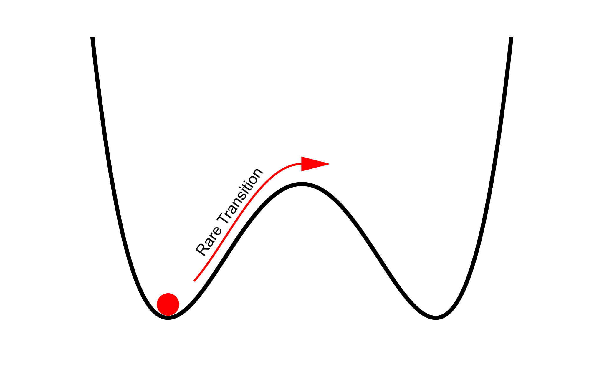
The basic idea is to add noise to this system which mimics the physical (thermal) fluctuations, and gather statistical information in the long time limit. The rare event which I am interested in occurs when the particle spontaneously jumps from one low energy basin to the other over the barrier.

Trajectories: Simulating Forward in Time

Adding noise to the system and watching the system evolve forward in time, \(t\), generates what is referred to as a trajectory. This trajectory is initialized at a user defined starting position, \(x_0\), and ends at some other position after \(N\) total time steps, generating a sequence of positions, \(\{x_0,x_1,x_2,\dotsc ,x_N\}\). An example of this procedure is shown in the following animation:

The left figure shows a particle (red dot), bouncing around in a double-well potential. The initial position of this example is at the minimum of the left well, where \(x_0 = x^-\). The trajectory associated with the motion is shown on in the right figure.

Properties of a Trajectory

1. Initial condition is defined (input as \(x_0\))
2. All trajectories (in a single simulation) have the same duration in time \(T=N~\Delta t\), where \(N\) is the number of samples generated.
3. The ending position, \(x_N\), cannot be defined a priori. For a large enough \(N\), the endpoints should be distributed according to the posterior probability distribution (Boltzmann in this case).

The major disadvantage of using trajectories to sample rare events is related to property 3. When the temperature (Noise) is small compared to the barrier separating the low energy basins, the amount of computational effort required to observe a (rare) transition event exponentially increases. This becomes a huge problem for more complicated systems where the most interesting events are extremely rare.

Double-Ended Paths: Adding Boundary Conditions

One approach to rectify this problem is to rewrite the equations of motion as a Stochastic Partial Differential Equation (SPDE), and impose boundary conditions on the beginning and end of the ‘trajectory’. This new object is referred to as a path, and requires a different type of sampling than the standard trajectory approach.

At face value, the major advantage of using a double-ended path over a trajectory is that rare events can be forced to occur by setting the boundaries to start in one well and end in another. Each path is then required to sample the (rare) transition event.

Properties of a Path

1. Boundary conditions are defined (starting at \(x_0\) and ending at \(x_N\)).
2. All paths have the same duration (T).
3. paths ‘evolve’ in path-time \(\tau\). At each path-time step, \(\Delta \tau\), an entire path must be defined.

The below animation serves to graphically represent what path sampling entails. At each path-time step, \(\Delta \tau\), a new path is generated in its entirety, starting with red and generating blue, then cyan and so on.

Now all that is left is to figure out how to perform the sampling with these paths, and what types of mathematical tricks are appropriate to apply when sampling diffusive Brownian motion.

Details of Path Sampling

Brownian Dynamics

Before moving to path sampling, lets start by writing the equation of motion for this noisy system. This dynamics can be described using a damped driven equation of motion \[\frac{dp}{d\tilde{t}} = F(x) - \gamma p + \text{Noise}\] where \(p\) is the momentum and \(F=-\frac{dV}{dx}\) is the Force on the particle. The Noise is defined using the Wiener process, \(dW_t\), which is scaled to the correct temperature, \(\epsilon\), using the fluctuation-dissipation theorem.

The systems of interest here reside in the over-damped Langevin regime (Brownian), where all particles have reached terminal velocity (\(dp/d\tilde{t} \rightarrow 0\)). With the substitution of a new algorithmic time, \(\tilde{t} = \gamma m t\), which is scaled by the mass (\(m\)) and the frictional coefficient (\(\gamma\)), the Langevin form of this equation is readily seen

\[dx = F(x) dt + \sqrt{2 \epsilon} d W_t\]

This Stochastic Differential Equation is defined in the form of a continuous time process. In order to numerically analyze the problem, a discretized form of the equation of motion is needed. The simplest (arguably) way to discretize this equation is given according to the Euler-Maryuama method, where the Weiner process has been approximated by a random Gaussian variate \(\xi\)

\[x_{i+1} = x_i + F(x_i) \Delta t + \sqrt{2 \epsilon \Delta t} \xi_i \label{forwardSDE}\]

Simply iterating this equation forward in time forms the canonical procedure to generate a Brownian trajectory.

Hybrid Monte Carlo

To create a more efficient algorithm, I have adapted the Hybrid Monte-Carlo method of Duane [1] for use with double ended paths. Using HMC dramatically increases the sampling efficiency over other standard methods like leapfrog or Metropolis Adjusted Langevin Algorithm (and other simple methods such as Random Walk Metropolis) as these methods sample the state space diffusively. The HMC method combines the strengths of 3 separate algorithms

1. Single Stochastic Step: Similar to the Euler-Maryuama method in Equation \(\ref{forwardSDE}\) and the Random Walk Metropolis algorithm, but adapted for use with double ended paths. This step is crucial, as it introduces randomness (noise) to the system, allowing access to all of phase space. The disadvantage of this step is it is entirely diffusive, which destroys the collective movements of the paths.
2. Multiple Molecular Dynamics (MD) Steps: This is where the majority of the path evolution occurs. These deterministic integrations can move large chunks of the path around in phase space. It is important to note that this integration can be handled exactly, as it is simply a deterministic Hamiltonian flow. This allows the high frequency modes to be integrated exactly and avoids subtraction of large numbers, thus reducing error and allowing the use of a larger algorithmic step size (\(\Delta \tau\)).
3. Metropolis Hastings Monte-Carlo (MHMC): The Stochastic and MD calculations above cannot, in general, be performed exactly. The MHMC test is used to correct for any errors made in these steps and drive the probability distribution to stationarity.

A crucial property of the HMC algorithm is the probability distribution is only modified in the first (Stochastic) step. The choice of random momenta (noise), importantly drawn to correspond to the Boltzmann distribution, will not necessarily leave the probability invariant, but all other steps will. The numerical integration of the Hamiltonian flow is symplectic and thus conserves phase space. The rejections in the Metropolis-Hastings step is needed to preserve detailed balance. These two together ensure that the algorithm samples the target probability distribution.

The question still remains: Why does the sampling improve on the original Brownian dynamics? As stated previously, introducing a Hamiltonian flow between the Brownian dynamics and the Metropolis test serves to dramatically increase the movement in phase space. These coordinate changes have a magnitude comparable to the standard deviation of the motion in the most highly constrained direction. That is, the changes are constrained to be approximately the square root of the smallest eigenvalue of the covariance matrix. Configurations which are not highly constrained benefit the most from the ballistic Hamiltonian flow [2].

Path Probability

Using the result of Onsager and Machlup  [3], one can quantify the probability of any double ended path. This is done by looking at the underlying random fluctuations of the paths themselves, which is given via the Gaussian random numbers \(\xi\). The probability of any path is given as

\[ - \ln \mathbb{P_{OM}} \propto \sum_i \frac{\xi_i^2}{2} = \frac{\Delta t}{2 \epsilon} \sum_i \frac{1}{2} \left| \frac{x_{i+1} - x_i}{\Delta t} - F(x_i) \right|^2 \label{eqn:OM}\]

The methods shown I am developing attempt to sample double ended paths which obey this probability.

Choice of Limiting Procedure

In order to perform accurate sampling, the limit where \(\Delta t\) is small must be examined. There are two ways to go about this

1. Continuous time limit (\(\Delta t \rightarrow dt\))
2. Small but finite \(\Delta t\)

Continuous Time Limit

In the continuous time limit the path probability  [4] [5] is derived using the Ito calculus and the Girsanov theorem to yield a surprisingly nice expression. Here, I write the regularized probability (regularized by the probability of the free motion (ie. when the force is zero), which is denoted by \(\mathbb{P}_0\)) and sample using the path space HMC method [6]

\[-\ln \frac{\mathbb{P}_{ITO}}{\mathbb{P}_0} \propto \frac{1}{2 \epsilon} \int_0^T dt \left( \frac{1}{2} \left| F(x) \right|^2 - \epsilon \nabla^2 V(x) \right) \label{eqn:ItoProb} \]

Implication: This probability distribution states that some paths are more probable than others. This is a violation of equilibrium thermodynamics! The results shown later confirm this.

Finite Time Limit

An alternative to the continuous time limit is to simply expand the original OM path probability in Equation \(\ref{eqn:OM}\). This expression is based on the Leap-Frog (velocity-Verlet) integrator applied to the HMC algorithm described previously.

\[-\ln \mathbb{P} \propto \frac{\Delta t}{2 \epsilon} \sum_i \left( \frac{1}{4} \left| \frac{x_{i+1} - x_i}{\Delta t} + F(x_{i+1}) \right|^2 + \frac{1}{4} \left| \frac{x_{i} - x_{i+1}}{\Delta t} - F(x_{i}) \right|^2 - \frac{\delta e_i}{\Delta t} \right) \label{eqn:FiniteProb}\]

Here,the last term is the error in energy per time step, which is given as

\[\frac{\delta e_i}{\Delta t} = \frac{V(x_{i+1}) - V(x_i)}{\Delta t} + \frac{x_{i+1} - x_i}{\Delta t} \frac{F(x_{i+1}) + F(x_i)}{2} + \frac{1}{4} \left( F(x_{i+1})^2 - F(x_i)^2 \right) \label{eqn:deltae}\]

There are two noteworthy comments to be made about this expression for the probability. First, the energy error made in this specific sampling violates detailed balance along the path. Second, in the limit where \(\Delta t \rightarrow 0\) and under the assumption that the noise is independent from the underlying potential (violated in the continuous time path probability shown in Equation \(\ref{eqn:ItoProb}\)), the quadratic variation, \(\Delta x^2 \rightarrow 2 \epsilon \Delta t\), is satisfied. By assuming the error along the path is negligible (\(\delta e \rightarrow 0\)), the cross terms in Equation \(\ref{eqn:deltae}\) reduce to the continuous time result

\[\frac{1}{2} \frac{\Delta x_i}{\Delta t} (F(x_{i+1}) - F(x_i)) \rightarrow \frac{1}{2} \frac{\Delta x_i^2}{\Delta t}{\Delta F_i}{\Delta x_i} \rightarrow \epsilon \nabla F\]

Now lets look at the sequence of paths which are generated by sampling in each of these limits.

Results

1D Entropic Potential

I will use a simple one dimensional potential to illustrate some results of these sampling methods. The potential is constructed to be degenerate in energy, but have wells of different widths. Entropy should then drive the particle to spend more time in the broad well than the narrow, according to the underlying Boltzmann probability. The Broad-Narrow potential is defined to be

\[V(x) = \frac{((8-5x)^8 ~ (2+5x)^2)}{2^{26}}\]

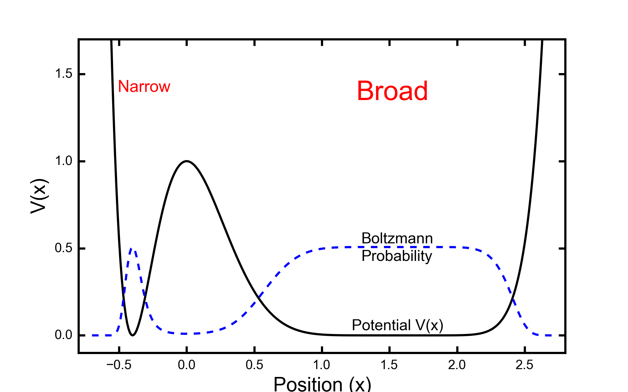
This potential has degenerate minima at \(x=-2/5\) and \(x=8/5\) with a barrier of height \(E_B\) equal to unity. The simulation performed at a configurational temperature of \(\epsilon = 0.25\), which gives a probability of the particle being in the wider well of \(\mathbb{P}(x>0) \approx 0.9\).

Path Evolution

In order to concisely present the evolution of paths generated using these two limits of the path sampling algorithm, I have calculated the fraction of each path which is contained in the broad well. I use the Heaviside function \(\Theta\) to calculate this fraction as follows

\[B(s) = \frac{1}{T} \int_0^T dt ~ \Theta(x_t^{(s)}) \approx \frac{1}{N} \sum_i \Theta(x_i^{(s)})\]

where the sampling index is denoted with s, and the corresponding path is \(\{x^{(s)} \}\). Let us now look at the results of the two path sampling algorithms:

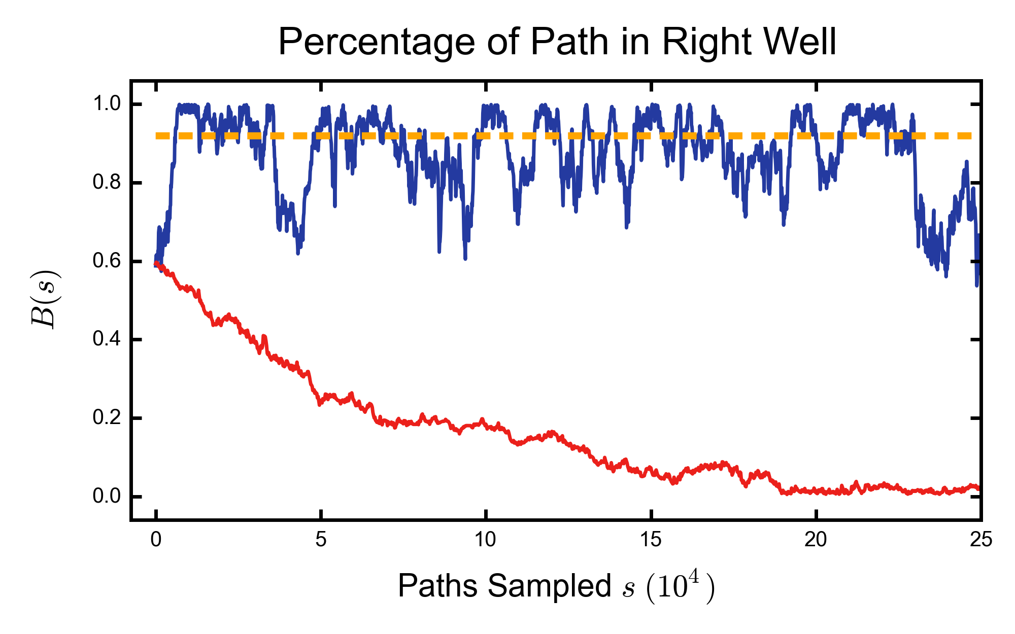
Here the yellow dotted line is the equilibrium (Boltzmann) value of \(B(s)\). The blue curve uses the finite time step probability and the red curve uses the continuous time representation.

The initial path was chosen to have approximately 60% of the path in the broad well, and has 3 separate transitions over the barrier. The final paths of the finite time step algorithm (Blue) are distributed in close proximity to the equilibrium value, but will only asymptotically approach the true value as \(\Delta t\) is decreased. The final paths of the continuous time representation (Red) is catastrophically incorrect, the paths spend the vast majority of time in the narrow (entropically confined) well.

The sampling can be seen in much greater detail in the below animations:

Continuous Time Limit: Path Evolution

Finite Time Limit: Path Evolution

Conclusions

Barrier hopping occurs rarely, but these hops are still consistent with equilibrium thermodynamics, and are observed in real life systems. Other, extremely rare events, while still allowed by statistical mechanics, are so rare that they violate thermodynamics. An example of such an event is all of the molecules in the air in the room you are sitting in moving to a single corner at the same time. For the paths of interest in this study, we expect to recover equilibrium thermodynamics, rather than all statistically allowed states.

Using the probability which comes from the continuous time limit leads to unphysical paths which are forced into the narrow well, which is not consistent with entropic considerations. This effect can be traced back to the form of the probability in Equation \(\ref{eqn:ItoProb}\). The noise originates from the thermal bath and is fully independent of the details of the deterministic force. The continuous time probability implies that some paths are more probable than others, which violates this independence.

Furthermore, sampling with this probability introduces correlation between the noise (fluctuations) and the positions along the path. This skews the velocity distribution and produces a non-Maxwell-Boltzmann velocity distribution.

Thus, this research shows that the continuous time formulation of the path probability in Equation \(\ref{eqn:ItoProb}\) cannot be used as a probability measure to sample physical paths.

On the other hand, the finite time representation of this probability measure generates paths which are consistent with the Boltzmann probability. The HMC picture explicitly describes the errors made in the approximate quadrature which are hidden in the Brownian picture. These errors manifest themselves as a simple numerical error (Equation \(\ref{eqn:deltae}\)) which is easily quantified.

References

[1] S. Duane, A. D. Kennedy, B. J. Pendleton, and D. Roweth, Physics Letters B 195, 216 (1987).
[2] R. Neal, Handb. Markov Chain Monte Carlo 113 (2011).
[3] S. Machlup and L. Onsager, Phys. Rev. 91, 1512 (1953).
[4] D. Dürr and A. Bach, Commun.Math. Phys. 60, 153 (1978).
[5] R. Graham, Z Physik B 26, 281 (1977).
[6] A. Beskos, F. J. Pinski, J. M. Sanz-Serna, and A. M. Stuart, Stochastic Processes and Their Applications 121, 2201 (2011).